Stainless steel components operating at elevated temperature - superheater tubes, reformer tubing, furnace headers - slowly deform and eventually fracture under sustained stress even when that stress is well below the material's short-term yield strength. This slow failure mode is called creep, and predicting when a component will rupture is essential to planning inspections, setting run lengths, and deciding when to retire or replace equipment.

This guide explains creep rupture behavior in stainless steel, how the Larson-Miller parameter converts scattered time-temperature test data into a usable design curve, and how that same parameter supports Remaining Life Assessment (RLA) for equipment already in service.
What Is Creep Rupture in Stainless Steel Components?
Creep rupture is the fracture of a stainless steel component after a period of slow, time-dependent deformation under constant load at elevated temperature, and it becomes a governing failure mode once metal temperature exceeds roughly 40–50% of the material's absolute melting point.
Below that temperature threshold, stainless steel components are designed against yield and tensile strength, and stress alone determines whether a part survives. Above it, time enters the equation: a stress level that a component could carry indefinitely at room temperature may cause it to slowly elongate, thin, and eventually fracture after months or years at high temperature, even though the stress never exceeds the material's rated allowable.
Creep progresses through three recognizable stages - primary creep (decelerating strain rate as the material work-hardens), secondary or steady-state creep (a roughly constant, minimum strain rate that dominates most of the component's life), and tertiary creep (accelerating strain rate as internal damage, cavitation, and cross-sectional loss drive the part to rupture). Because most of a component's service life is spent in the steady-state stage, engineers use that stage's data to predict total time to rupture.
What Is the Larson-Miller Parameter and How Is It Calculated?
The Larson-Miller Parameter (LMP) is a single numerical value that combines absolute temperature and rupture time into one term, allowing creep test data collected at high temperature over short durations to predict rupture life at lower service temperatures over much longer durations.
The parameter is defined as:
LMP = T × (C + log₁₀ tᵣ)
where T is the absolute temperature (in Rankine or Kelvin), tᵣ is the time to rupture in hours, and C is a material-specific constant - commonly close to 20 for austenitic stainless steels, though it is fitted from test data for each alloy. The elegance of the parameter is that, for a given stress level, tests run at different temperature and time combinations that share the same LMP value will fail at essentially the same stress.
This means a laboratory can run short-duration tests at high temperature and use the resulting LMP-versus-stress curve to predict rupture life at a lower service temperature over a much longer time - spans that would otherwise take years or decades to test directly.
The constant C shifts the curve horizontally and is not universal: it depends on the alloy's metallurgy and must be derived from a regression fit of that alloy's own rupture data rather than assumed from another material. Using the wrong C value for a given stainless grade produces a systematically shifted - and unreliable - rupture-life estimate, which is why published reference curves (ASME, API) specify C alongside the LMP-stress relationship for each grade.
How Do You Use the Larson-Miller Parameter to Predict Creep Rupture Life?
Rupture life is predicted by locating the operating stress on a material's published LMP-versus-stress master curve, reading off the corresponding LMP value, and then solving the Larson-Miller equation for time at the component's actual operating temperature.

The process runs in three steps. First, determine the operating (or design) stress on the component, typically from hoop stress in a pressure-retaining tube or vessel wall. Second, use the alloy's published master curve - a plot of stress versus LMP built from a large database of rupture tests - to find the LMP value that corresponds to that stress.
Third, rearrange the Larson-Miller equation to solve for rupture time at the actual service temperature: tᵣ = 10^[(LMP/T) − C]. Because temperature sits inside the equation as an absolute value multiplying the whole bracket, small increases in metal temperature produce disproportionately large reductions in predicted rupture life - a relationship covered in more detail in the next section.
A simplified worked illustration
- Determine hoop stress at the tube wall from operating pressure, diameter, and wall thickness.
- Read the LMP value corresponding to that stress from the grade's master curve (for example, TP321H).
- Solve tᵣ = 10^[(LMP/T) − C] using the component's actual absolute metal temperature.
- Compare the calculated rupture time to elapsed and planned future service hours to judge margin.
How Does Temperature Affect Creep Rupture Life Compared to Stress?
Because temperature multiplies the entire Larson-Miller bracket while stress only shifts position along the master curve, a relatively small sustained increase in metal temperature - as little as 15–25°C (about 30–50°F) above design - can cut remaining creep life by half or more, making temperature control the single most sensitive variable in creep-limited service.
This sensitivity is why hot-spot temperature excursions, localized flame impingement, or insulation damage are disproportionately dangerous in creep-limited equipment: a component running just a few percent hotter than intended is not aging a few percent faster - it may be aging several times faster. This nonlinearity is also why continuous or periodic metal-temperature monitoring is treated as a primary input to remaining life assessment, often weighted more heavily than stress-side variables such as minor pressure fluctuations, in an operating unit.
Which Stainless Steel Grades Are Most Susceptible to Creep, and Which Resist It Best?
Standard austenitic grades such as TP304H, TP316H, TP321H, and TP347H all deliver useful creep strength up to roughly 800–840°C (1470–1545°F), with the higher-alloyed 316H and 347H offering somewhat better high-temperature performance than 304H, while nickel-iron-chromium alloys like 800H/HT extend usable creep life several hundred degrees further for the most severe furnace and reformer service.

Creep resistance in these grades comes primarily from solid-solution strengthening (chromium, nickel, molybdenum) and, in the stabilized "H" grades, controlled carbon content and grain size that resist premature carbide coarsening at temperature. TP321H and TP347H add titanium or niobium stabilization, which improves resistance to sensitization during long, cyclic high-temperature exposure - a metallurgical benefit distinct from, but often paired with, creep strength.
Beyond the practical ceiling of standard austenitic stainless steels, nickel-based alloys take over because their higher nickel content further slows diffusion-controlled creep mechanisms at temperatures where iron-based austenitic structures begin to lose strength rapidly.
Typical Larson-Miller constants and practical service ceilings for common creep-resistant grades:
|
Stainless Grade |
Typical LMP Constant C |
Practical Service Ceiling |
Typical Application |
|
TP304H / 304H |
≈ 20 |
≈ 800–815°C (1470–1500°F) |
Superheater and reheater tubing, moderate creep duty |
|
TP316H / 316H |
≈ 20 |
≈ 815–840°C (1500–1545°F) |
Higher-temperature superheater tubing, refinery furnace tubes |
|
TP321H |
≈ 20 |
≈ 800–815°C (1470–1500°F) |
Cyclic high-temperature service where sensitization resistance matters |
|
TP347H |
≈ 20 |
≈ 815–840°C (1500–1545°F) |
Long-term high-temperature headers and superheaters |
|
Alloy 800H/HT (nickel-iron-chromium) |
≈ 15–17 |
≈ 900–980°C (1650–1800°F) |
Ethylene furnace tubing, high-temperature reformer service |
Table 1. Representative Larson-Miller constants and service ceilings for common creep-resistant stainless and nickel-iron-chromium grades. Values are illustrative; always confirm against the current edition of ASME II-D or the applicable material specification before use in design or fitness-for-service calculations.
What Is Remaining Life Assessment (RLA) and When Should It Be Performed?
Remaining Life Assessment is an engineering evaluation - combining inspection data, operating history, and creep-life models like the Larson-Miller parameter - that estimates how much useful service life a component has left, and it should be performed on any creep-exposed component approaching its original design life, after a known temperature excursion, or at scheduled turnaround intervals for units running at or near creep-range temperatures.
An RLA typically combines several lines of evidence rather than relying on the Larson-Miller calculation alone: recorded operating temperature and pressure history, wall-thickness and dimensional measurements from inspection, microstructural evaluation (replication or metallography looking for creep cavitation and voids), and hardness or other nondestructive indicators of material degradation.
The Larson-Miller-based calculation establishes a theoretical, model-based rupture life; physical inspection evidence - particularly creep cavitation observed by metallographic replication - either confirms that estimate or reveals that actual damage has progressed faster or slower than the model predicts, which is why codes such as API 579-1/ASME FFS-1 treat calculated life and inspected condition as complementary, not interchangeable, inputs.
How Is the Larson-Miller Parameter Used in a Remaining Life Assessment?
In an RLA, the Larson-Miller parameter is used to convert a component's full temperature and time operating history into cumulative consumed creep life, most commonly through a life-fraction (Robinson's rule) summation that adds up the fraction of rupture life used in each distinct operating period.

Because service conditions rarely hold constant, assessors break the operating history into discrete time-temperature-stress intervals, calculate the predicted rupture life for each interval using the Larson-Miller relationship, and express each interval as a fraction of that predicted life (actual hours at that condition divided by predicted rupture hours at that condition).
Summing these fractions across the component's full history gives the cumulative life fraction consumed; when that sum approaches 1.0, the component is approaching its statistically predicted rupture point under a linear damage assumption. Because this summation is sensitive to exactly the temperature data discussed above, the reliability of an RLA's output depends heavily on the quality and resolution of the underlying temperature history - sparse or estimated temperature records widen the uncertainty band substantially more than sparse stress records do.
What Are the Limitations and Common Pitfalls of the Larson-Miller Method?
The Larson-Miller method is a statistically fitted extrapolation tool, not a physical damage measurement, so its accuracy degrades when applied outside the temperature-stress range of the underlying test data, when the wrong constant C is used, or when it is treated as a standalone answer instead of one input alongside physical inspection.
Common pitfalls include extrapolating well beyond the tested stress-temperature envelope, where the master curve's uncertainty widens considerably; applying a generic literature constant C to a specific heat or product form without validating it against that material's actual chemistry and grain structure; ignoring multiaxial stress states or weld and heat-affected-zone effects, which often have different - typically lower - creep strength than base metal; and using the Larson-Miller life-fraction result in isolation without corroborating physical evidence such as metallographic replication or dimensional survey.
Because the underlying test database represents average behavior across many heats, the method is best used to establish expected life and inspection intervals, with confirmed physical condition governing the final fitness-for-service decision on any specific component.
How Do I Choose Between Larson-Miller and Other Creep Life Prediction Methods?
Larson-Miller is the right default choice for most stainless steel applications because it requires the fewest fitted constants and is directly supported by codified reference curves in ASME and API, while Manson-Haferd and Orr-Sherby-Dorn are reserved for cases where LMP shows systematic curvature across a wide temperature range or where a research-grade activation-energy basis is preferred.
All three time-temperature parameters solve the same underlying problem - converting scattered short-term, high-temperature test data into a usable long-term, lower-temperature prediction - but they differ in mathematical form and data requirements, summarized below.
|
Criterion |
Larson-Miller (LMP) |
Manson-Haferd |
Orr-Sherby-Dorn |
|
Governing form |
P = T(C + log t) |
P = (log t − log tₐ) / (T − Tₐ) |
P = log t − Q / (2.3RT) |
|
Number of fitted constants |
One (C) |
Two (tₐ, Tₐ) |
One (activation energy Q) |
|
Typical use in stainless steels |
Most widely published; ASME/API reference curves use C ≈ 20 |
Used where LMP shows curvature across wide temperature ranges |
Common in academic/metallurgical creep studies |
|
Data needed to fit the constant |
Minimal - published C values available for standard grades |
Requires a broader multi-temperature test matrix |
Requires known or fitted activation energy |
|
Extrapolation risk |
Moderate - well-validated within tested stress/temperature range |
Lower within its fitted range, higher outside it |
Sensitive to accuracy of Q |
|
Industry adoption for RLA |
Dominant - ASME B31.3, API 579-1/ASME FFS-1 reference LMP curves |
Occasional, refinery/power niche use |
Primarily research, limited codified use |
Table 2. Comparison of common time-temperature parameter methods for creep rupture life prediction.
For most stainless steel piping, pressure vessel, and tubing applications, Larson-Miller is sufficient and is the method embedded in widely used reference sources, which is itself a practical reason to default to it: assessments built on a codified, widely reviewed method are easier to defend in an inspection or fitness-for-service review than one built on a less common parameter.
Frequently Asked Questions
What is a safe starting point for the Larson-Miller constant C for stainless steel?
A value of approximately 20 is a commonly cited starting point for austenitic stainless steels such as 304H, 316H, 321H, and 347H, but it should always be verified against the specific material specification or test data rather than assumed, since actual fitted values can vary by alloy and product form.
Can the Larson-Miller parameter be used for welds and heat-affected zones?
Only with a separate, weld-specific master curve; weld metal and heat-affected zones commonly exhibit different - often lower - creep rupture strength than base metal, so base-metal LMP curves should not be applied directly to weld locations without adjustment or dedicated weld creep data.
How often should a Remaining Life Assessment be repeated?
Frequency is typically tied to calculated remaining life and criticality: components with a large calculated life fraction remaining may be reassessed at normal turnaround intervals, while components approaching a life fraction near 1.0, or that experienced a known over-temperature event, warrant more frequent reassessment and closer inspection.
Does the Larson-Miller parameter apply to fatigue as well as creep?
No. The Larson-Miller parameter is specifically a creep-rupture (time-dependent, sustained-load) model; cyclic fatigue damage from repeated stress or thermal cycling is evaluated with separate fatigue methods, and components subject to both mechanisms typically require a combined creep-fatigue interaction assessment.
What single data quality issue most undermines a Larson-Miller-based RLA?
Incomplete or estimated metal temperature history, because temperature has a disproportionately large effect on calculated rupture life compared with stress; an RLA built on sparse or assumed temperature data carries substantially wider uncertainty than one built on continuous, measured records.